Line Fitting Using Gaussian Loopy Belief Propagation
Gaussian Belief Propagation is a variant of Belief Propagation and used for inference on graphical models if the underlying distribution is described as a Gaussian.
This article describes the implementation of the inference of a piecewiese separated Line using Gaussian Loopy Belief Propagation. The example is taken from A visual introduction to Gaussian Belief Propagation. I work here with a stripped version of Joseph Ortiz’s notebook in hope to make the implementation more comprehensible. My contribution is to explain what is going on in the code and relate it to the formulas and algorithms given in the introduction as the notebook contains mostly only code (as of now).
Please use the original notebook, if you want to experiment. It provides a very nice framework and you might want to use the functions I have deleted.
Please see also my other articles on the topic, if you are not familiar with Belief Propagation. They provide very simple implementations of where discrete distributions are used.
- Loopy Belief Propagation - Python Implementation
- Simple Noise Reduction with Loopy Belief Propagation
Implementation
Imports
import numpy as np
import torch
import random
import os
import matplotlib.pyplot as plt
from typing import List, Callable, Optional, Union
%matplotlib inline
Gaussian Component
We store here the gaussian component using the canonical parameters \(\eta\) and \(\Lambda\).
The relation to the \(\mu\) (mean) and \(\Sigma\) (covariance) is:
\[\Lambda = \Sigma^{-1} \qquad \text{and} \qquad \eta = \Lambdaμ\]"""
This is a single Gaussian defined with canonical parameters eta and lambda.
"""
class Gaussian:
def __init__(self, dim: int, eta: Optional[torch.Tensor]=None, lam: Optional[torch.Tensor]=None, type: torch.dtype = torch.float):
"""
Initializes the Gaussian
dim: dimension of the Gaussian
eta: is the related to the mean (canonical)
lam: is the precision matrix (inverse of the covariance)
type: datatype of one cell
"""
self.dim = dim
if eta is not None and eta.shape == torch.Size([dim]):
self.eta = eta.type(type)
else:
self.eta = torch.zeros(dim, dtype=type)
if lam is not None and lam.shape == torch.Size([dim, dim]):
self.lam = lam.type(type)
else:
self.lam = torch.zeros([dim, dim], dtype=type)
def mean(self) -> torch.Tensor:
"""
computes the mean based on eta and lambda
"""
return torch.matmul(torch.inverse(self.lam), self.eta)
def cov(self) -> torch.Tensor:
"""
computes and returns the covariance by the inverse of lambda
"""
return torch.inverse(self.lam)
def mean_and_cov(self) -> List[torch.Tensor]:
"""
computes the covariance by the inverse of lambda
computes the mean based on eta and lambda
returns both
"""
cov = self.cov()
mean = torch.matmul(cov, self.eta)
return [mean, cov]
def set_with_cov_form(self, mean: torch.Tensor, cov: torch.Tensor) -> None:
"""
set eta and lambda using the given mean and covariance
"""
self.lam = torch.inverse(cov)
self.eta = self.lam @ mean
Loss functions
We define two loss functions here. Squared or quadratic error loss and Huber loss. This is to see the different effects for the different loss functions.
You’ll find in the section Factor Node how the loss function is used.
"""
    Defines squared error loss functions that correspond to Gaussians.
    Robust losses are implemented by scaling the Gaussian covariance.
"""
class SquaredLoss():
    def __init__(self, dofs: int, diag_cov: Union[float, torch.Tensor]) -> None:
        """
            dofs: degrees of freedom (dimension) of the measurement
            diag_cov: diagonal elements of covariance matrix
        """
        assert diag_cov.shape == torch.Size([dofs])
        mat = torch.zeros(dofs, dofs, dtype=diag_cov.dtype)
        mat[range(dofs), range(dofs)] = diag_cov
        self.cov = mat
        self.effective_cov = mat.clone()

    def get_effective_cov(self, residual: torch.Tensor) -> None:
        """ Set the covariance of the Gaussian (squared loss) that matches the loss at the error value. """
        self.effective_cov = self.cov.clone()

    def robust(self) -> bool:
        return not torch.equal(self.cov, self.effective_cov)


class HuberLoss(SquaredLoss):
    def __init__(self, dofs: int, diag_cov: Union[float, torch.Tensor], stds_transition: float) -> None:
        """
            stds_transition: num standard deviations from minimum at which quadratic loss transitions to linear
        """
        SquaredLoss.__init__(self, dofs, diag_cov)
        self.stds_transition = stds_transition

    def get_effective_cov(self, residual: torch.Tensor) -> None:
        mahalanobis_dist = torch.sqrt(residual @ torch.inverse(self.cov) @ residual)
        if mahalanobis_dist > self.stds_transition:
            self.effective_cov = self.cov * mahalanobis_dist**2 / (2 * self.stds_transition * mahalanobis_dist - self.stds_transition**2)
        else:
            self.effective_cov = self.cov.clone()

"""
    The measurement model defines how to relate a measurement to a prediction
"""
class MeasModel:
    def __init__(self, meas_fn: Callable, jac_fn: Callable, loss: SquaredLoss, *args) -> None:
        """
            Initializes the measurement model
            meas_fn: measurement functions that defines how to relate a measurement to a prediction
            jac_fn: if the measurement function is not linear we need a linearization function. This is called jacobian function here
            loss: loss function
        """
        self._meas_fn = meas_fn
        self._jac_fn = jac_fn
        self.loss = loss
        self.args = args
        self.linear = True

    def jac_fn(self, x: torch.Tensor) -> torch.Tensor:
        """
            Returns the computed jacobian
            x: linearization point
        """
        return self._jac_fn(x, *self.args)

    def meas_fn(self, x: torch.Tensor) -> torch.Tensor:
        """
            Returns the measurement generating point
            x: measurement
        """
        return self._meas_fn(x, *self.args)
Settings
These are only global setting for the Gaussian belief propagation.
class GBPSettings:
    def __init__(self,
                 damping: float = 0.,
                 beta: float = 0.1,
                 num_undamped_iters: int = 5,
                 min_linear_iters: int = 10,
                 dropout: float = 0.,
                 reset_iters_since_relin: List[int] = [],
                 type: torch.dtype = torch.float) -> None:

        # Parameters for damping the eta component of the message
        self.damping = damping
        # Number of undamped iterations after relinearisation before damping
        # is set to damping
        self.num_undamped_iters = num_undamped_iters

        self.dropout = dropout

        #
        # Parameters for just in time factor relinearisation
        #

        # Threshold absolute distance between linpoint and adjacent belief
        # means for relinearisation.
        self.beta = beta
        # Minimum number of linear iterations before a factor is
        # allowed to relinearise.
        self.min_linear_iters = min_linear_iters
        self.reset_iters_since_relin = reset_iters_since_relin

    def get_damping(self, iters_since_relin: int) -> float:
        if iters_since_relin > self.num_undamped_iters:
            return self.damping
        else:
            return 0.
Factor Graph
The factor graph is the container for all nodes, factors and variables. It allows to add any kind of factor, like smoothing and measurement, by defining arbitrary measurement functions.
The function gbp_solve executes
robustify_all_factorsRescale the variance of the noise in the Gaussian measurement model, if necessary and update the factors correspondinglyjit_linearisationto relinearize the factors, if the measurement model is not linearcompute_all_messagesto compute all outgoing messages from factorsupdate_all_beliefsto compute the belief for each node
for each iteration.
class FactorGraph:
    def __init__(self, gbp_settings: GBPSettings = GBPSettings()) -> None:
        self.var_nodes = []
        self.factors = []
        self.gbp_settings = gbp_settings

    def add_var_node(self,
                    dofs: int,
                    prior_mean: Optional[torch.Tensor] = None,
                    prior_diag_cov: Optional[Union[float, torch.Tensor]] = None,
                    properties: dict = {}) -> None:
        """
            Add a variable node to the network
            dofs: degrees of freedom (dimensions) of the variable node
        """
        variableID = len(self.var_nodes)
        self.var_nodes.append(VariableNode(variableID, dofs, properties=properties))
        if prior_mean is not None and prior_diag_cov is not None:
            prior_cov = torch.zeros(dofs, dofs, dtype=prior_diag_cov.dtype)
            prior_cov[range(dofs), range(dofs)] = prior_diag_cov
            self.var_nodes[-1].prior.set_with_cov_form(prior_mean, prior_cov)
            self.var_nodes[-1].update_belief()

    def add_factor(self, adj_var_ids: List[int],
                    measurement: torch.Tensor,
                    meas_model: MeasModel,
                    properties: dict = {}) -> None:
        """
            Add a factor to the network
            measurement: the measurement that is associated to the factor
            meas_model: measurement model to relate the measurement to nodes
            properties: additional properties (optional) that can be used in the factors
        """

        factorID = len(self.factors)
        adj_var_nodes = [self.var_nodes[i] for i in adj_var_ids]
        self.factors.append(Factor(factorID, adj_var_nodes, measurement, meas_model, properties=properties))
        for var in adj_var_nodes:
            var.adj_factors.append(self.factors[-1])

    def update_all_beliefs(self) -> None:
        """
            This is the product of all incoming messages from all
            adjacent factors for node.
        """
        for var_node in self.var_nodes:
            var_node.update_belief()

    def compute_all_messages(self, apply_dropout: bool = True) -> None:
        for factor in self.factors:
            if apply_dropout and random.random() > self.gbp_settings.dropout or not apply_dropout:
                damping = self.gbp_settings.get_damping(factor.iters_since_relin)
                factor.compute_messages(damping)

    def linearise_all_factors(self) -> None:
        for factor in self.factors:
            factor.compute_factor()

    def robustify_all_factors(self) -> None:
        for factor in self.factors:
            factor.robustify_loss()

    def jit_linearisation(self) -> None:
        """
            This is executed only if the measurement model is not linear.
            Check for all factors that the current estimate is close to
            the linearisation point.
            If not, relinearise the factor distribution.
            Relinearisation is only allowed at a maximum frequency of once
            every min_linear_iters iterations.
        """
        for factor in self.factors:
            if not factor.meas_model.linear:
                adj_belief_means = factor.get_adj_means()
                factor.iters_since_relin += 1
                if torch.norm(factor.linpoint - adj_belief_means) > self.gbp_settings.beta and \
                        factor.iters_since_relin >= self.gbp_settings.min_linear_iters:
                    factor.compute_factor()

    def synchronous_iteration(self) -> None:
        """
            One iteration
        """
        self.robustify_all_factors()
        self.jit_linearisation()  # For linear factors, no compute is done
        self.compute_all_messages()
        self.update_all_beliefs()

    def gbp_solve(self, n_iters: Optional[int] = 20, converged_threshold: Optional[float] = 1e-6, include_priors: bool = True) -> None:
        """
            Main function to for inference
            n_iters: maximum number of iterations
            converged_threshold: difference of energy of after an iteration
        """
        energy_log = [self.energy()]
        print(f"\nInitial Energy {energy_log[0]:.5f}")
        i = 0
        count = 0
        not_converged = True
        while not_converged and i < n_iters:
            self.synchronous_iteration()
            if i in self.gbp_settings.reset_iters_since_relin:
                for f in self.factors:
                    f.iters_since_relin = 1

            energy_log.append(self.energy(include_priors=include_priors))
            print(
                f"Iter {i+1}  --- "
                f"Energy {energy_log[-1]:.5f} --- "
                # f"Belief means: {self.belief_means().numpy()} --- "
                # f"Robust factors: {[factor.meas_model.loss.robust() for factor in self.factors]}"
                # f"Relins: {sum([(factor.iters_since_relin==0 and not factor.meas_model.linear) for factor in self.factors])}"
                  )
            i += 1
            if abs(energy_log[-2] - energy_log[-1]) < converged_threshold:
                count += 1
                if count == 3:
                    not_converged = False
            else:
                count = 0

    def energy(self, eval_point: torch.Tensor = None, include_priors: bool = True) -> float:
        """ Computes the sum of all of the squared errors in the graph using the appropriate local loss function. """
        if eval_point is None:
            energy = sum([factor.get_energy() for factor in self.factors])
        else:
            var_dofs = torch.tensor([v.dofs for v in self.var_nodes])
            var_ix = torch.cat([torch.tensor([0]), torch.cumsum(var_dofs, dim=0)[:-1]])
            energy = 0.
            for f in self.factors:
                local_eval_point = torch.cat([eval_point[var_ix[v.variableID]: var_ix[v.variableID] + v.dofs] for v in f.adj_var_nodes])
                energy += f.get_energy(local_eval_point)
        if include_priors:
            prior_energy = sum([var.get_prior_energy() for var in self.var_nodes])
            energy += prior_energy
        return energy

    def belief_means(self) -> torch.Tensor:
        """ Get an array containing all current estimates of belief means. """
        return torch.cat([var.belief.mean() for var in self.var_nodes])

    def belief_covs(self) -> List[torch.Tensor]:
        """ Get a list containing all current estimates of belief covariances. """
        covs = [var.belief.cov() for var in self.var_nodes]
        return covs

    def print(self, brief=False) -> None:
        print("\nFactor Graph:")
        print(f"# Variable nodes: {len(self.var_nodes)}")
        if not brief:
            for i, var in enumerate(self.var_nodes):
                print(f"Variable {i}: connects to factors {[f.factorID for f in var.adj_factors]}")
                print(f"    dofs: {var.dofs}")
                print(f"    prior mean: {var.prior.mean().numpy()}")
                print(f"    prior covariance: diagonal sigma {torch.diag(var.prior.cov()).numpy()}")
        print(f"# Factors: {len(self.factors)}")
        if not brief:
            for i, factor in enumerate(self.factors):
                if factor.meas_model.linear:
                    print("Linear", end =" ")
                else:
                    print("Nonlinear", end =" ")
                print(f"Factor {i}: connects to variables {factor.adj_vIDs}")
                print(f"    measurement model: {type(factor.meas_model).__name__},"
                    f" {type(factor.meas_model.loss).__name__},"
                    f" diagonal sigma {torch.diag(factor.meas_model.loss.effective_cov).detach().numpy()}")
                print(f"    measurement: {factor.measurement.numpy()}")
        print("\n")
Variable Node
A variable node consists of
- id
- optional properties (a dict, to store additional values)
- degrees of freedom (dimension of the Gaussian component)
- references to adjacent factors
- its belief, which is a Gaussian component
- a prior, which is also a Gaussian component
The belief of the node is updated with update_belief. It takes the product of all incoming messages, which is implemented as a sum of the \(\eta\) and a sum of the \(\Lambda\) of the outgoing messages from the adjacent factors to a variable node.
The function get_prior_energy computes the engergy which can also be seen as as the negative log likelihood of the residual between the variable belief mean and the prior mean.
class VariableNode:
    def __init__(self, id: int, dofs: int, properties: dict = {}) -> None:
        self.variableID = id
        self.properties = properties
        self.dofs = dofs
        self.adj_factors = []
        self.belief = Gaussian(dofs)
        # prior factor, implemented as part of variable node
        self.prior = Gaussian(dofs)

    def update_belief(self) -> None:
        """
            Update local belief estimate by taking product of all
            incoming messages along all edges.
        """
        self.belief.eta = self.prior.eta.clone()  # message from prior factor
        self.belief.lam = self.prior.lam.clone()

        # messages from other adjacent variables
        for factor in self.adj_factors:
            message_ix = factor.adj_vIDs.index(self.variableID)
            self.belief.eta += factor.messages[message_ix].eta
            self.belief.lam += factor.messages[message_ix].lam

    def get_prior_energy(self) -> float:
        energy = 0.
        if self.prior.lam[0, 0] != 0.:
            residual = self.belief.mean() - self.prior.mean()
            energy += 0.5 * residual @ self.prior.lam @ residual
        return energy
Factor Node
Consists of:
- id
- degrees of freedom
- adjacent variable nodes
- outgoing messages modeled as Gaussian components. One for each adjacent variable.
- a factor (a Gaussian component)
- a linearization point (a vector of the size the degrees of freedom, initialized with zero)
- a measurement
- the measurement model
- additional properties
The degrees of freedom of a factor node is the sum of the degrees of freedom of adjacent variable nodes.
compute_factor
The function compute_factor computes, as the name says, the \(\eta\) and \(\Lambda\) of the factor. This is done first at initialization and after a certain number of iterations if the measurement model is not linear.
First, we need the linearization point \(\mu\). This is the concatenated mean of the beliefs of the adjacent variable nodes.
The Jacobian \(J\) is computed using the Jacobian function of the the given measurement model. The linearization point \(\mu\) is given for general purposes. We won’t need this argument in our line fitting example below.
Next, the predicted measurement \(x\) is computed by the measurement model given the linearization point \(\mu\). Please see below in the Line Fitting section how the measurement model and linearization function are defined.
The loss function is provided as a covariance \(\Sigma_L\).In case of Huber loss we need the residual \(x - z\), where \(z\) is the measurement attached to the factor, to get the effective loss. The residual doesn’t play any role in case the squared loss is used. The unchanged loss covariance is used then. As the Gaussian are computed in canonical form we need the inverse of the covariance \(\Sigma_L\), which is the precision matrix \(\Lambda_L\).
The new \(\Lambda_f\) and \(\eta_f\) for the factor are then:
\[\Lambda_L = \Sigma_L^{-1}\] \[\Lambda_f = J^T \Lambda_L J\] \[\eta_f = (J^T \Lambda_L) (J \mu + z - x)\]compute_messages
All outgoing messages to the variable nodes are computed by compute_messages
The factor-to-variable message is given by
\[\mu_{f \to x}(x) = \sum_{\chi_f \setminus x}\phi_f(\chi_f) \prod_{y \in \{ne(f) \setminus x \}} \mu_{y \to f}(y)\]where \(\phi_f(\chi_f)\) is the probability distribution associated with the factor, and \(\sum_{\chi_f \setminus x}\) sums over all variables except \(x\) which is called marginalization.
First, we have to compute the product of the factor with all incoming messages from the adjacent variable nodes except the one coming from the variable node \(x\).
Consider a factor \(f\) is connected to two variable nodes \(x_1\) and \(x_2\). We want to compute the message to \(x_1\). The Gaussian parameters of the factor are then:
\[\eta_f = \begin{bmatrix} \eta_{f_1} \\ \eta_{f_2} \end{bmatrix} \qquad \text{and} \qquad \Lambda_f = \begin{bmatrix} \Lambda_{f_{11}} & \Lambda_{f_{12}} \\ \Lambda_{f_{21}} & \Lambda_{f_{22}} \end{bmatrix}\]We take the product of the factor distribution and the message coming from the other adjacent variables node to the factor as follows.
\[\eta_f' = \begin{bmatrix} \eta_{f_1} \\ \eta_{f_2} + \eta_{x_2 \to f} \end{bmatrix} \qquad \text{and} \qquad \Lambda_f' = \begin{bmatrix} \Lambda_{f_{11}} & \Lambda_{f_{12}} \\ \Lambda_{f_{21}} & \Lambda_{f_{22}} + \Lambda_{x_2 \to f} \end{bmatrix}\]The \(\eta_{x_i \to f}\) is the \(\eta\) of the i’th variable node belief minus the \(\eta\) of the respective outgoing message from the factor to the i’th variable node. Similarly \(\Lambda_{x_i \to f}\) is the difference of the \(\Lambda\) of the i’th variable node belief and the \(\Lambda\) of the respective outgoing message from the factor to the i’th variable node.
In the second step we have to marginalize out all variables except \(x_1\), which is the receiving node. The marginalization of Gaussian distributions is described in Pattern Recognition and Machine Learning by Bishop. See 2.3.2 Marginal Gaussian distributions page 88. The canonical form is given by Ryan M. Eustice et. al. Exactly Sparse Delayed-State Filters
Given a joint distribution of the variables \(x_a\) and \(x_b\) with the parameters
\[\eta = \begin{bmatrix} \eta_a \\ \eta_b \end{bmatrix} \qquad \text{and} \qquad \Lambda = \begin{bmatrix} \Lambda_{aa} & \Lambda_{ab} \\ \Lambda_{ba} & \Lambda_{bb} \end{bmatrix}\]\(b\) is marginalized out using
\[\bar{\eta_a} = \eta_a - \Lambda_{ab} \Lambda_{bb}^{-1} \eta_{b} \qquad \text{and} \qquad \bar{\Lambda_a} = \Lambda_{aa} - \Lambda_{ab} \Lambda_{bb}^{-1} \Lambda_{ba}\]This requires in general to reorder \(\eta_f'\) and \(\lambda_f'\) to have the output variable on top.
class Factor:
    def __init__(self,
                 id: int,
                 adj_var_nodes: List[VariableNode],
                 measurement: torch.Tensor,
                 meas_model: MeasModel,
                 type: torch.dtype = torch.float,
                 properties: dict = {}) -> None:

        self.factorID = id
        self.properties = properties

        self.adj_var_nodes = adj_var_nodes
        self.dofs = sum([var.dofs for var in adj_var_nodes])
        self.adj_vIDs = [var.variableID for var in adj_var_nodes]
        self.messages = [Gaussian(var.dofs) for var in adj_var_nodes]

        self.factor = Gaussian(self.dofs)
        self.linpoint = torch.zeros(self.dofs, dtype=type)

        self.measurement = measurement
        self.meas_model = meas_model

        # For smarter GBP implementations
        self.iters_since_relin = 0

        # compute the factor
        self.compute_factor()

    def get_adj_means(self) -> torch.Tensor:
        """
            concatenates the mean values (vectors) of the adjacent
            variable beliefs. Such as
            [MeanOfBeliefOfNode1, MeanOfBeliefOfNode1] is
            [tensor([1., 2.]), tensor([3., 4.])]
            becomes
            tensor([1., 2., 3., 3.])
        """
        adj_belief_means = [var.belief.mean() for var in self.adj_var_nodes]
        return torch.cat(adj_belief_means)

    def get_residual(self, eval_point: torch.Tensor = None) -> torch.Tensor:
        """
            Compute the residual vector.
            This is the difference between the result of a given measurement
            function on a evaluation point and a measurement.
            The evaluation point is the concatenated mean of the
            adjacent variables belief, if the evaluation point is not given
            as a parameters.
        """
        if eval_point is None:
            eval_point = self.get_adj_means()
        return self.meas_model.meas_fn(eval_point) - self.measurement

    def get_energy(self, eval_point: torch.Tensor = None) -> float:
        """
            Computes the squared error using the appropriate loss function.
            The engery can be interpreted as the negative log likelihood
            of the residual using the inverse of the effective covariance
            of the given loss function.
        """
        residual = self.get_residual(eval_point)
        # print("adj_belifes", self.get_adj_means())
        # print("pred and meas", self.meas_model.meas_fn(self.get_adj_means()), self.measurement)
        # print("residual", self.get_residual(), self.meas_model.loss.effective_cov)
        return 0.5 * residual @ torch.inverse(self.meas_model.loss.effective_cov) @ residual

    def robust(self) -> bool:
        return self.meas_model.loss.robust()

    def compute_factor(self) -> None:
        """
            Compute the factor at current adjacente beliefs.
            If measurement model is linear then factor will always be the same
            regardless of linearisation point.
        """
        self.linpoint = self.get_adj_means()
        J = self.meas_model.jac_fn(self.linpoint)
        pred_measurement = self.meas_model.meas_fn(self.linpoint)
        self.meas_model.loss.get_effective_cov(pred_measurement - self.measurement)
        effective_lam = torch.inverse(self.meas_model.loss.effective_cov)
        self.factor.lam = J.T @ effective_lam @ J
        self.factor.eta = ((J.T @ effective_lam) @ (J @ self.linpoint + self.measurement - pred_measurement)).flatten()
        self.iters_since_relin = 0

    def robustify_loss(self) -> None:
        """
            Rescale the variance of the noise in the Gaussian measurement model
            if necessary and update the factor correspondingly.
        """
        old_effective_cov = self.meas_model.loss.effective_cov[0, 0]
        self.meas_model.loss.get_effective_cov(self.get_residual())
        self.factor.eta *= old_effective_cov / self.meas_model.loss.effective_cov[0, 0]
        self.factor.lam *= old_effective_cov / self.meas_model.loss.effective_cov[0, 0]

    def compute_messages(self, damping: float = 0.) -> None:
        """ Compute all outgoing messages from the factor. """

        # temporary outgoing messages
        messages_eta, messages_lam = [], []

        start_dim = 0

        # iterate over all adjacent variables
        # v is the variable node we want to compute the outgoing message
        for v in range(len(self.adj_vIDs)):
            # get a copy of eta and lambda with double precision from
            # this factor
            eta_factor, lam_factor = \
                self.factor.eta.clone().double(), \
                self.factor.lam.clone().double()

            # Iterate over all adjacent variabel nodes except the one
            # we want to compute the outgoing message.
            # Take the product of factor with incoming messages.
            # This is done by adding the residual messages to respective
            # cells of the factor.
            start = 0
            for var in range(len(self.adj_vIDs)):
                if var != v:
                    var_dofs = self.adj_var_nodes[var].dofs
                    eta_factor[start:start + var_dofs] += \
                        self.adj_var_nodes[var].belief.eta - \
                        self.messages[var].eta
                    lam_factor[start:start + var_dofs, start:start + var_dofs] += \
                        self.adj_var_nodes[var].belief.lam - \
                        self.messages[var].lam

                start += self.adj_var_nodes[var].dofs

            #
            # Divide up parameters of distribution
            #
            # In order to compute the marginal we have to rearrage
            # the eta and the lambda
            #

            # Dimensions of the outgoing message
            mess_dofs = self.adj_var_nodes[v].dofs
            # eta for a (output - which goes on top)
            eo = eta_factor[start_dim:start_dim + mess_dofs]
            # eta for b (which goes on to the bottom)
            eno = torch.cat((eta_factor[:start_dim], eta_factor[start_dim + mess_dofs:]))

            # the lambda has four parts
            # top left (output) - lambda_aa (loo), top right lambda_ab (lono),
            # bottom left - lambda_ba (lnoo),      bottom right - lambda_bb (lnono)

            loo = lam_factor[start_dim:start_dim + mess_dofs, start_dim:start_dim + mess_dofs]
            lono = torch.cat((lam_factor[start_dim:start_dim + mess_dofs, :start_dim],
                              lam_factor[start_dim:start_dim + mess_dofs, start_dim + mess_dofs:]), dim=1)
            lnoo = torch.cat((lam_factor[:start_dim, start_dim:start_dim + mess_dofs],
                              lam_factor[start_dim + mess_dofs:, start_dim:start_dim + mess_dofs]), dim=0)
            lnono = torch.cat(
                        (
                            torch.cat((lam_factor[:start_dim, :start_dim], lam_factor[:start_dim, start_dim + mess_dofs:]), dim=1),
                            torch.cat((lam_factor[start_dim + mess_dofs:, :start_dim], lam_factor[start_dim + mess_dofs:, start_dim + mess_dofs:]), dim=1)
                        ),
                        dim=0
                    )

            # Marginalization
            new_message_lam = loo - lono @ torch.inverse(lnono) @ lnoo
            new_message_eta = eo - lono @ torch.inverse(lnono) @ eno
            # Add the new output message
            messages_eta.append((1 - damping) * new_message_eta + damping * self.messages[v].eta)
            messages_lam.append((1 - damping) * new_message_lam + damping * self.messages[v].lam)
            start_dim += self.adj_var_nodes[v].dofs

        for v in range(len(self.adj_vIDs)):
            self.messages[v].lam = messages_lam[v]
            self.messages[v].eta = messages_eta[v]
Line Fitting
How Guassian belief propagation works is shown here on the example of piecewise linear function fitting. We place in equal distance a number of variable nodes along the x-axis. Each node is defined as a one dimensional gaussian component. Its mean is the height or y-position. A number of random measurement that follow a noisy sinus curve are used to estimate the beliefs of the nodes.
Create custom factors
We we create two types of factors. One for smoothing the mean of adjacent nodes \(x\) and one that incorporates the height measurement. Each factor is connected to two adjacent nodes.
The predicted mean is computed with the height measurement function. It takes the height of the belief of the adjacent nodes and uses the \(\gamma\) (a scalar) to compute the new mean.
\(J = [1 - \gamma, \gamma]\) \(\bar{\mu} = J \mu\)
where \(\gamma\) is the the relative distance in x-direction of the measurement \(z\) to left nearest variable node.
\[\gamma = \frac{z^{(x)} - x_i^{(x)}}{x_{i+1}^{(x)} - x_{i}^{(x)}}\]The Jacobian of the height measurement model is just \(J\) and is linear.
The measurement model for smoothing computes just the difference between the mean of two adjacent variable nodes.
def height_meas_fn(x: torch.Tensor, gamma: torch.Tensor):
    """
        computes the y-position by summing scaled y-position of
        two adjacent variable nodes. Based on this y-position the residual
        can be computed
        x: y-positions of two adjacent nodes
        gamma: a scaling factor
    """
    J = torch.tensor([[1-gamma, gamma]])
    return J @ x

def height_jac_fn(x: torch.Tensor, gamma: torch.Tensor):
    """
        computes the jacobian which are only the scaling factors
        for the two adjacent variable nodes
        x: y-positions of two adjacent nodes
        gamma: a scaling factor
    """
    return torch.tensor([[1-gamma, gamma]])

class HeightMeasurementModel(MeasModel):
    def __init__(self, loss: SquaredLoss, gamma: torch.Tensor) -> None:
        MeasModel.__init__(self, height_meas_fn, height_jac_fn, loss, gamma)
        self.linear = True

def smooth_meas_fn(x: torch.Tensor):
    return torch.tensor([x[1] - x[0]])

def smooth_jac_fn(x: torch.Tensor):
    return torch.tensor([[-1., 1.]])

class SmoothingModel(MeasModel):
    def __init__(self, loss: SquaredLoss) -> None:
        MeasModel.__init__(self, smooth_meas_fn, smooth_jac_fn, loss)
        self.linear = True
Global parameters
n_varnodes = 20       # number of variables
x_range = 10          # data range
n_measurements = 15   # number of measurements

gbp_settings = GBPSettings(
    damping = 0.1,
    beta = 0.01,
    num_undamped_iters = 1,
    min_linear_iters = 1,
    dropout = 0.0,
  )

# Gaussian noise measurement model parameters:
prior_cov = torch.tensor([10.]) # the prior covariance of the variable nodes
data_cov = torch.tensor([0.05]) # the covariance of the measurement
smooth_cov = torch.tensor([0.1])
data_std = torch.sqrt(data_cov)
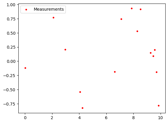
Measurements
The height of the measurement follow a noisy sinus curve.
# Plot measurements
meas_x = torch.rand(n_measurements)*x_range
meas_y = torch.sin(meas_x) + torch.normal(0, torch.full([n_measurements], data_std.item()))
plt.scatter(meas_x, meas_y, color="red", label="Measurements", marker=".")
plt.legend()
plt.show()
Create factor graph
fg = FactorGraph(gbp_settings)
# The x-coordinates of the variable nodes
xs = torch.linspace(0, x_range, n_varnodes).float().unsqueeze(0).T
# add a variables nodes with y-position zero and the given prior covarance
for i in range(n_varnodes):
fg.add_var_node(1, torch.tensor([0.]), prior_cov)
# add a smoothing factor to each node except the last
for i in range(n_varnodes-1):
fg.add_factor(
[i, i+1], # adjacent variable ids
torch.tensor([0.]), # measurement (empty)
SmoothingModel(SquaredLoss(1, smooth_cov)) # Smoothing model
)
# add a measurement factor to each node except the last
for i in range(n_measurements):
# we are attaching one measurement to a factor.
# Each factor is attached to the two adjacent
# variable nodes
ix2 = np.argmax(xs > meas_x[i])
ix1 = ix2 - 1
# This is a scaling factor to interpolate the y-coordinate (the means)
# between two adajacent variable nodes nodes. This is: The closer
# a measurement is positioned to a variable node, the more
# we trust its y-position.
# The distance in x-direction between measurement and node ix1
# divided by the distance in x-direction of the two variable
# nodes gives the scaling factor
gamma = (meas_x[i] - xs[ix1]) / (xs[ix2] - xs[ix1])
fg.add_factor(
[ix1, ix2],
meas_y[i],
HeightMeasurementModel(
SquaredLoss(1, data_cov),
gamma
)
)
fg.print(brief=True)
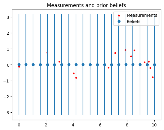
# Beliefs are initialized to zero
# Plot beliefs and measurements
covs = torch.sqrt(torch.cat(fg.belief_covs()).flatten())
plt.title("Measurements and prior beliefs")
plt.errorbar(xs, fg.belief_means(), yerr=covs, fmt='o', color="C0", label='Beliefs')
plt.scatter(meas_x, meas_y, color="red", label="Measurements", marker=".")
plt.legend()
plt.show()
Factor Graph:
# Variable nodes: 20
# Factors: 34
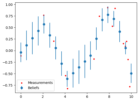
Solve with GBP
fg.gbp_solve(n_iters=50)

# Plot beliefs and measurements
covs = torch.sqrt(torch.cat(fg.belief_covs()).flatten())
plt.errorbar(xs, fg.belief_means(), yerr=covs, fmt='o', color="C0", label='Beliefs')
plt.scatter(meas_x, meas_y, color="red", label="Measurements", marker=".")
plt.legend()
plt.show()
Initial Energy 49.21330
Iter 1  --- Energy 27.81385 ---
Iter 2  --- Energy 23.62700 ---
Iter 3  --- Energy 20.39776 ---
Iter 4  --- Energy 16.08122 ---
Iter 5  --- Energy 13.77354 ---
Iter 6  --- Energy 13.69291 ---
Iter 7  --- Energy 13.48928 ---
Iter 8  --- Energy 13.46488 ---
Iter 9  --- Energy 13.43425 ---
Iter 10  --- Energy 13.42690 ---
Iter 11  --- Energy 13.42052 ---
Iter 12  --- Energy 13.41977 ---
Iter 13  --- Energy 13.41866 ---
Iter 14  --- Energy 13.41855 ---
Iter 15  --- Energy 13.41835 ---
Iter 16  --- Energy 13.41833 ---
Iter 17  --- Energy 13.41829 ---
Iter 18  --- Energy 13.41828 ---
Iter 19  --- Energy 13.41828 ---
Iter 20  --- Energy 13.41828 ---
Iter 21  --- Energy 13.41827 ---
Iter 22  --- Energy 13.41827 ---
Iter 23  --- Energy 13.41827 ---
Iter 24  --- Energy 13.41827 ---
Iter 25  --- Energy 13.41827 ---
Iter 26  --- Energy 13.41827 ---
References
- A visual introduction to Gaussian Belief Propagation by Joseph Ortiz, Talfan Evans and Andrew J. Davison
- Loopy Belief Propagation - Python Implementation by me on this blog
- Simple Noise Reduction with Loopy Belief Propagation by me on this blog
- Pattern Recognition and Machine Learning by Christopher M. Bishop.
- Exactly Sparse Delayed-State Filters by Ryan M. Eustice et. al.