Simple Noise Reduction with Loopy Belief Propagation
I want to continue my previous post with a (useful) example to get more a feel how to use Loopy Belief Propagation in practice.
The aim is to remove noise from an image - which is only a toy example.
Please see the References. I have taken the ideas from there. My contribution is only to give an example of their work coded in python for learning purposes.
Graph
The graph is initialy defined as Markov Random Field (MRF). Like the one below.

The black circles are the observed nodes \(y_i\). These are the noisy pixels of an image. We want to infer the latent variable \(x_i\) for each of the observed nodes. Which are the denoised pixels and depicted as a white circles. The connections of the \(x_i\) to the neighbors are made because the change of color from pixel to pixel is considered sparse. One pixel may tell its neighbor the belief of its color. Please see Loopy Belief Propagation in Image-Based Rendering by Dana Sharon for a detailed explanation.
We turn now the MRF into a loopy factor graph.

The white circles remain the hidden variables we want to infer. The black circles are turned now into squares colored in black. These are factors and related to a probabilty of the observations. The white squares are factors that define how neigboring pixels are related.
Variables and Factors
I will use a binary black and white picture in order to simplify the computation and ease the understanding. Thus all the variables are binary and the factors may consists only of a two-by-two matrix.
A variable is defined by
\[x_{ij} = \begin{pmatrix} p(white) \\ p(black) \\ \end{pmatrix}\]It contains for row \(i\) and column \(j\) a probability that the pixel is black or white.
The factor colored in white is defined by:
\[\psi_{kl}^h = \begin{pmatrix} s_{remains\_white}(x) & s_{changes\_to\_black}(x)\\ s_{changes\_to\_white}(x) & s_{remains\_black}(x) \\ \end{pmatrix}\]It gives a score for all possibilities a hidden variable may change or not change its color. The appropriate values will be defined later.
The factor colored in black is defined by:
\[\psi_{ij}^o = \begin{pmatrix} s(white) \\ s(black) \\ \end{pmatrix}\]This takes just the probability of the observed pixel. \(s(white)\) is \(0.6\) if the the pixel is white, \(s(white)\) is \(0.4\) if the observed pixel is black. And similarly for the score \(s(black)\). These values are just arbitrarily defined. One should find the true probabilities to improve the performance.
Python implementation
This implementation is naïve. It just aims to make things clear without the need of hiding the operations in optimizations.
Still I can simplify the code from previous post a little. I don’t want to use the named tensor concept here. Simply because the names would be meaningless in this example. And also products can be simplified as the factors are two dimensional at maximum. Summing over the product becomes a matrix to vector multiplication - which I have shown in the previous post. Please see the section Factor-to-Variable Message Example 1.
Graph implementation
The graph must reflect the structure of the lattice. The observed factor nodes are 2x1 arrays. We add them to a array in the size of the image. The hidden factors (non shaded) are 2x2 arrays. It turns out that we don’t need to reserve space in the lattice for these factors as they are everywhere the same. Defining only one is enough. For each observed pixel we need a variable that represents the final belief of a pixel. This can also be expressed with a 2x1 array. Last, each node is connected at maximum to four (unshaded) factors. That means we need at maximum four additional incoming messages and four outgoing messages, each of the size of a 2x1 array, for each node.
A node element can be defined with an array containing 9 messages and 1 marginal, where each element is a 2x1 array like this:
array([[[0.],  # Variable marginal
        [0.]],

       [[0.],  # Observed factor incoming message
        [0.]],

       [[0.],  # Upper incoming message
        [0.]],

       [[0.],  # Upper outgoing message
        [0.]],

       [[0.],  # Left incoming message
        [0.]],

       [[0.],  # Left outgoing message
        [0.]],

       [[0.],  # Lower incoming message
        [0.]],

       [[0.],  # Lower outgoing message
        [0.]],

       [[0.],  # Right incoming message
        [0.]],

       [[0.],  # Right outgoing message
        [0.]]])
import numpy as np
from enum import IntEnum
class MsgType(IntEnum):
    MARGINAL = 0
    OBSERVED = 1
    NEIGHBOR = 2

n_rows = 100     # number of image rows
n_cols = 100     # number of image columns
n_messages = 10  # number of elements to describe a node
n_dims = 2       # element dimension

# The graph
# All messages are intialized with [0.5, 0.5].Transpose
graph = np.ones(n_rows * n_cols * n_messages * n_dims).reshape(n_rows, n_cols, n_messages, 2, 1) * 0.5
Loading an Image Into the Graph
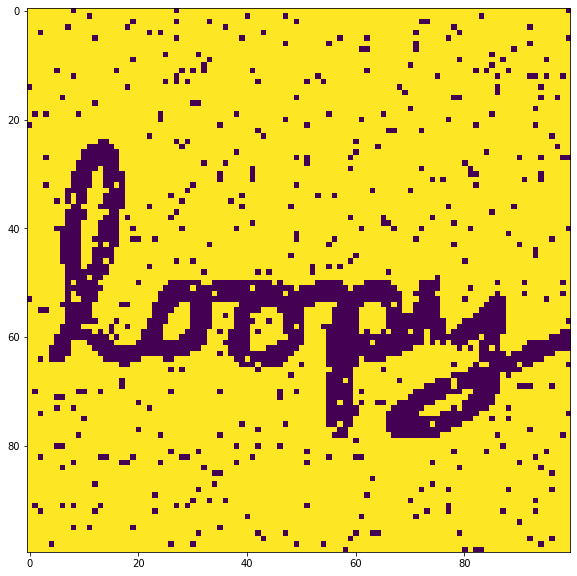
Lets load a self drawn 100 x 100 image, add some noise and convert it to a binary image.
from matplotlib import pyplot as plt
from skimage import io
from skimage.color import rgb2gray
from skimage.color import rgba2rgb
import skimage

loopy_image_array_rgb = io.imread('https://raw.githubusercontent.com/mayio/mayio.github.io/master/docs/_posts/2022-09-24-Noise-Reduction-Loopy-Belief-Propagation_files/loopy.png')
loopy_image_array_rgb = skimage.util.random_noise(loopy_image_array_rgb, mode='pepper')
loopy_image_array_gray = rgb2gray(rgba2rgb(loopy_image_array_rgb));
loopy_image_array_bw =  (loopy_image_array_gray > 0.5) + 0.;

fig = plt.figure(figsize=(15, 10))
plt.imshow(loopy_image_array_bw)
plt.show()
The pixel values must be loaded into the incoming message of the “observed” factors. We reduce the probability a bit, as we are not shure about the right value.
for i in range(n_rows):
    for j in range(n_cols):
        pixel_value = loopy_image_array_bw[i][j]
        graph[i][j][MsgType.OBSERVED][0][0] = pixel_value * 0.2 + 0.4
        graph[i][j][MsgType.OBSERVED][1][0] = (1. - pixel_value) *  0.2 + 0.4
Message Computation
The variable-to-factor message is given by:
\[\mu_{x \to f}(x) = \prod_{g \in \{ne(x) \setminus f\}} \mu_{g \to x}(x)\]where \(ne(x)\) are the neighbors of \(x\).
And the factor-to-variable message is given by
\[\mu_{f \to x}(x) = \sum_{\chi_f \setminus x}\phi_f(\chi_f) \prod_{y \in \{ne(f) \setminus x \}} \mu_{y \to f}(y)\]See below how this is implemented for the lattice.
Variable to Factor
The incoming messages of a variable (coming from the hidden (unshaded) and observed (shaded) factors) are simply multiplied element-wise, excluding the incoming message from the factor we want to send the message to.
You will find a normaliziation in the code below. That is actually not needed. But without we would run into numerical problems as the multiplication makes the values small. One would compute these values rather in log-space to avoid numerical problems.
For a given variable and message we may do:
def variable_to_factor_message(i, j, k, max_rows, max_cols):
    # get the indices for the neighboring node
    i2 = i - 1 if k == 0 else i   # top
    i2 = i + 1 if k == 2 else i2  # bottom
    j2 = j + 1 if k == 1 else j   # left
    j2 = j - 1 if k == 3 else j2  # right

    # check the neighboring node exists
    if i2 < 0 or j2 < 0 or i2 >= max_rows or j2 >= max_cols:
      return

    # get the variable
    variable = graph[i][j]

    # get the observed incoming factor
    res = np.copy(variable[MsgType.OBSERVED])

    # iterate through all neigbors except the given k
    # do a element-wise product
    for l in range(4):
      if l != k:
        res  = res * variable[MsgType.NEIGHBOR + l * 2]

    # store the result in the outgoing message
    norm = res[0][0] + res[1][0]
    variable[MsgType.NEIGHBOR + k * 2 + 1][:] = res / norm
Factor to Variable
The hidden factors are indirectly accessed. We have to find the neighboring nodes and access the respective messages. If we have the right messages, we may do a simple matrix to vector multiplication here. There is even no need to transpose the factor depending on the edge direction as the factor is a symetric matrix.
Again, the normalization is actually not needed. One might choose the sum of log-likelihoods for the product and use the log-sum-exp trick for the summation.
hidden_factor = np.array([[0.6, 0.4],[0.4, 0.6]])

def factor_to_variable_message(i1, j1, k1, max_rows, max_cols):
    # get the indices for the neighboring node
    i2 = i1 - 1 if k1 == 0 else i1  # top
    i2 = i1 + 1 if k1 == 2 else i2  # bottom
    j2 = j1 + 1 if k1 == 1 else j1  # left
    j2 = j1 - 1 if k1 == 3 else j2  # right

    # check the neighboring node exists
    if i2 < 0 or j2 < 0 or i2>= max_rows or j2 >= max_cols:
        return

    # this node
    variable_receive = graph[i1][j1];

    # neighboring node
    variable_source = graph[i2][j2];

    # the opposite edge - the index of the outgoing message of
    # the neighboring node
    k2 = (k1 + 2) % 4

    # matrix multiplication of hidden factor with the outgoing message
    # of the neighboring node
    variable_receive[MsgType.NEIGHBOR + k1 * 2][:] = np.matmul(
        hidden_factor,
        variable_source[MsgType.NEIGHBOR + k2 * 2 + 1])

    norm = sum(variable_receive[MsgType.NEIGHBOR + k1 * 2])[0]
    variable_receive[MsgType.NEIGHBOR + k1 * 2] /= norm
Marginal
The marginal of a variable is given by
\[p(x) \propto \prod_{f \in ne(x)}\mu_{f \to x}(x)\]This is very similar to the computation of the variable to factor message. Now we multiply all incoming messages element-wise.
def marginal(i, j, max_rows, max_cols):
    variable = graph[i][j];
    res = np.copy(variable[MsgType.OBSERVED])

    for k in range(4):
        # get the indices for the neighboring node
        i2 = i - 1 if k == 0 else i   # top
        i2 = i + 1 if k == 2 else i2  # bottom
        j2 = j + 1 if k == 1 else j   # left
        j2 = j - 1 if k == 3 else j2  # right

        # check the neighboring node exists
        if i2 < 0 or j2 < 0 or i2>= max_rows or j2 >= max_cols:
            continue

        # iterate through all neigbors
        # do a element-wise product
        res  = res * variable[MsgType.NEIGHBOR + k * 2]

    # store the result in the outgoing message
    norm = res[0][0] + res[1][0];
    variable[MsgType.MARGINAL][:] = res / norm
Inference
Now put everything together and run the inference. We iterate in multiple rounds over all variables, compute the variable-to-factor messages and then the factor-to-variables messages.
At last we compute the marginal for each variable. This is usually not needed in each iteration for most applications as only the final result is needed. In this toy example we want to show the intermediate results.
iterations = 4
loopy_image_array_update = np.copy(loopy_image_array_bw);

# create figure
fig = plt.figure(figsize=(15, 10))

for n_iter in range(iterations):
    # start with variable to factor message.
    for i in range(n_rows):
        for j in range(n_cols):
            # we have to iterate over all available neighbors of a variable
            for k in range(4):
                variable_to_factor_message(i, j, k, n_rows, n_cols)

    # continue with factor to variable message.
    for i in range(n_rows):
        for j in range(n_cols):
            # we have to iterate over all available neighbors of a variable
            # to compute all factor to variable messages
            for k in range(4):
                factor_to_variable_message(i, j, k, n_rows, n_cols)

    # marginal
    for i in range(n_rows):
        for j in range(n_cols):
            marginal(i, j, n_rows, n_cols)

    fig.add_subplot(1, iterations, n_iter + 1)

    for i in range(n_rows):
        for j in range(n_cols):
            loopy_image_array_update[i][j] = (np.argmax(graph[i][j][0]) - 1) * -1

    plt.imshow(loopy_image_array_update)

plt.show()
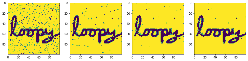
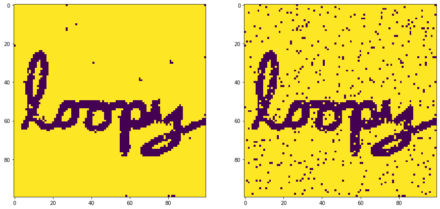
fig = plt.figure(figsize=(15, 10))
fig.add_subplot(1, 2, 1)
plt.imshow(loopy_image_array_update)
fig.add_subplot(1, 2, 2)
plt.imshow(loopy_image_array_bw)
plt.show()
References
- Understanding Belief Propogation and its Generalizations by Jonathan S. Yedidia, William T. Freeman, and Yair Weiss
- Loopy Belief Propagation in Image-Based Rendering by Dana Sharon
- Variational Inference: Loopy Belief Propagation by Eric P. Xing
- Stereo Matching with Loopy Belief Propagation blog